The Pavement Management Blog

Prepared by Magdy Mikhail, Texas Department of Transportation

Network-level structural data provides information about the load-carrying capacity of the pavement network. It describes base and surface strength, as well as subgrade strength. This information can be essential in determining whether a candidate project needs sub-surface rehabilitation or if a less expensive (surface) preventive maintenance treatment can be used instead.  The data can also be used for evaluating routes for super heavy loads.

Network level structural evaluation can be done using one of the available devices below:

• The Falling Weight Deflectometer (FWD) to assess structural capacity of pavements, data is collected every 0.3-0.5 miles by applying an impact load of 9,000 lb to simulate the  load of one tire of a single axle loaded to 18,000 lb. the deflection basin generated is suitable for structural evaluation.  The data is collected at a relatively slow rate and traffic control is always needed for the safety of the operator, equipment and travelling public.
• Rolling Wheel Deflectometer (RWD) device that uses two sensors to collect the maximum pavement surface deflection under an 18-kip single axle semi-trailer load traveling at normal highway speeds. The device provides high production suitable for network level evaluation and traffic control is not needed for data collection.
• Traffic Speed Deflectometer (TSD) which is a truck trailer combination having a 10 tonnes single axle with dual wheels. The movement of the pavement surface caused by the axle load is measured with four (or more) laser sensors and is transformed to simulate a deflection basin.  The equipment operates at highway speed without the need for traffic control.

 

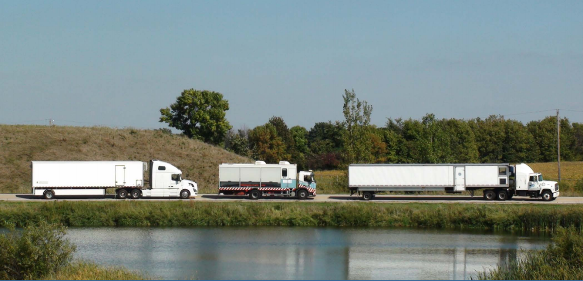
Continuous deflection testing devices at MnROAD test facility for an FHWA study on “Network Level Pavement Structural Evaluation”. From left to right: Greenwood TSD, Euroconsult Curviameter, and Applied Research Associates (ARA) RWD. [Picture Source: “Network Level Pavement Structural Evaluations – A Way forward,” Presented by Nadarajah Sivaneswaran (FHWA) at National Pavement Evaluation Conference 2014]

In general the data from the different equipment can be incorporated into a structural index to be used in the decision tree to generate preventive maintenance and rehabilitation plans and optimize the use of the available funds.

 

For more information, please contact Magdy Mikhail at: Magdy.Mikhail@txdot.gov

Prepared by Raja Shekharan, Virginia Department of Transportation

Maintenance of pavement network in an optimal condition has been increasingly becoming a necessity for various agencies. Individual pavement sections within a network are at different condition levels and require several different types of appropriate Maintenance and Rehabilitation (M&R) treatments. If the availability of funding for the maintenance of the network is not a concern, plausibly every pavement section needing a treatment could be provided with the treatment. In reality, there is rarely enough funding to cover the maintenance needs of an entire network, and most of the times the available funding can sufficiently address only a portion of the M&R needs of a network.

To use the limited funds in a cost-effective manner, various types of strategies and analysis procedures are adopted. As a strategy for network maintenance, a mix of fixes that includes pavement preservation, i.e., a spectrum of treatments ranging from lighter types such as preventive maintenance to heavier types such as reconstruction is adopted. Pavement preservation represents a proactive approach in maintaining pavements that reduces expensive heavier treatments and associated traffic disruptions while providing increased mobility and reduced congestion. Based on the existing structural and functional condition of pavements, there are windows of opportunity when particular types of treatments would be suitable. Established pavement management systems answer the questions of when, where, and what regarding the treatment types to be provided for various pavement sections. This makes it all the more important to not just address the worst sections but to use mix-of-fixes as a network level maintenance strategy. The lighter preventive type of treatments can be provided to those sections that are lightly distressed and require only functional conditions to be addressed while the heavier treatment types are to be provided for pavements that are heavily distressed requiring some kind of structural condition to be addressed. The lighter types of treatments are more economical on per unit basis and therefore can cover a larger portion of the network with a given amount of funding or a portion of that funding. Application of these lighter treatments to appropriate sections retards their deterioration into condition states needing costlier heavier treatments.

Heavier treatments are necessary to address heavily distressed pavements that cannot be properly addressed with lighter treatments. With a given funding level it may not be possible to address all the pavements in the network that need heavier treatments within one year. These sections need to be addressed over multiple years while other sections are provided with other appropriate treatments as a part of the network maintenance strategy. It is well recognized that using treatments as band-aids, wherein a lighter treatment is used as a temporary measure till the needed heavier treatment is applied, is not a part of pavement preservation strategy. It is also to be noted that providing heavier treatments are not cost-effective on sections requiring lighter treatments. On the other hand, providing lighter treatments are ineffective for sections when heavier treatments are warranted. This leads to a reemphasis of providing the right treatment to the right section at the right time for the optimal maintenance of a pavement network.

This article originally appeared in the International Journal of Pavement Research and Technology (IJPRT), Vol. 8, No. 1 issue, 2015. For more information, please contact Raja Shekharan at: Raja.Shekharan@VDOT.Virginia.gov

Prepared by Zhongren Wang, Caltrans

1. Introduction

A typical output from a Pavement Management System (PMS) is a list of recommended pavement improvement projects. These PMS-recommended projects need to be reviewed, adjusted, and finalized before possible funding commitment. In the review process, the relationships between the recommended projects and the currently programmed, under-construction, and as-built projects must be identified and closely examined to avoid gaps, overlaps, or inappropriate treatments. Presented in a tabular format, such a list of projects does not lend itself to easy identification of the necessary relationships. A visualization environment is necessary.

At the California Department of Transportation (Caltrans), the importance of such a visualization environment for project review has long been recognized. In the past, Caltrans pavement engineers manually drew horizontal bar charts using Microsoft Excel® for such purposes. Led by Tom Pyle, a Caltrans Supervising Transportation Engineer, the manually-drawn bar charts were further developed and automated in the process of implementing the Caltrans pavement management system, called PaveM. Present automation was developed through contract with the University of California Pavement Research Center (UCPRC). The product is called H-Chart, short for Highway chart. The following is a brief description of the H-chart.

 

2. H-Chart

An H-chart, as shown in Figure 1, provides the visualization of all past, current, and future projects for one direction of a specific route within one county, and one district. Caltrans divides its jurisdiction into 12 districts up and down California. For example, the H-chart shown in Figure 1 is dedicated for the northbound direction of route 101 in Del Norte County, in Caltrans District 01.

In Figure 1, the x-axis shows the county odometer and the y-axis shows Year. Projects are shown as hatched and colored horizontal bars. The project limits (the start and end locations) are located on the x-axis by means of county odometer values. These county odometer values are computed from the state odometer associated with the start and end of a project. The year of the project is indicated by its vertical location on the chart.

An H-chart displays projects with four different states, namely (1) Completed or as-built, (2) Under Construction, (3) Programmed, and (4) PMS- or PaveM-Recommended. These project states are indicated in the chart by different cross-hatching patterns. In an H-chart, the earliest known as-built projects are displayed at the bottom of page, followed by the programmed and under construction projects, and finally the recommended future projects at the top. The thick dashed horizontal line in Figure 1 separates the recommended future projects from the rest.

Each project shown in Figure 1 is also identified by a budget group. There are four budget groups for typical pavement projects in Caltrans. These include (1) Highway Maintenance (HM) Preventive, (2) HM Corrective programs, (3) Capital Program Maintenance (CAPM), and Rehabilitation. Each budget group is associated with a specific color. For example, Rehabilitation group is associated with red color.

Each project also has a label that contains such information as: treatment type, lane number or “All”, Expenditure Authorization (EA) number and Post-Mile (PM) limits.  The contents of the label are configurable when the H-charts are generated. Use the label in the upper left corner of Figure 1 “CinPlePrecyc-All 01-2T12LA-T-II” as an example, this label signifies that this particular project is a PaveM-recommended project with a Cold-in-Place-Recycling treatment for “All” lanes. The EA number of 01-2T12LAT is a temporary one (for future potential project with no funding commitment), because it ends with a capital letter ‘T’. As a rule, an EA number with funding commitment ends with a numeric value in Caltrans. For example, the label shown in Figure 1 “Med OL-All 01-49940” means a “Medium Overlay” treatment for all lanes with an EA number of “01-49940”. The “-II” following the EA number refers to the PaveM running Scenario that corresponds to the title of the chart.

Together with the depicted projects, pavement type and pavement condition information is also respectively shown at the top and bottom of the sample H-chart shown in Figure 1. The cracking and IRI values are based on the latest available pavement condition survey. The label for ‘crack%’, such as “0.3/2:0.7” shown at the lower left corner of Figure 1 means that the average wheel path cracking across all lanes from PM 0 to PM 4.4 is 0.3%, and the highest cracking percentage is 0.7%, occurring in lane number 2.

H-Charts are generated automatically with minimal post-processing in Excel®. A total of 1066 H-charts can be generated across the entire California pavement network based on the available district, county, route, and route direction combinations. The detailed breakdowns of these H-charts for each Caltrans district are tabulated in Table 1. Readers are encouraged to try out this web-based H-Chart generation application on their own. The website is: http://dev.ucprc.ucdavis.edu/PaveM-rViewer/.

 

Table 1. The Number of H-Charts for Each District and the State

District	1	2	3	4	5	6	7	8	9	10	11	12
Number	60	80	132	175	84	120	98	88	38	99	56	36
Total	1066

 

Figure 1 A Sample H-Chart (Please click on figure to see larger version)

 

3. How to Use an H-Chart?

With pavement condition, as-built projects, programmed projects, and PaveM-recommended projects visualized in one chart, an H-chart provides an effective working environment for pavement engineers to evaluate, compare, adjust, and select projects for future programming and planning purposes. An H-chart makes it easy to identify overlapping projects in schedule, or in limits. For example, project 01-49940 and 01-08080 shown in Figure 1 overlap in schedule. It may not make sense to apply a medium overlay treatment on top of a thin overlay treatment that just applied a year ago. An H-chart also facilitates the easy identification of project gaps. For example, the segment from PM 20 to 25 has not been treated ever since the year of 1994. Why is there such a long hiatus for a flexible pavement to be treated? Is it because of too low a traffic volume?  Is it due to short of funding? Or is it because the project history is not completely shown by the H-chart? Answers to these types of questions may well help better plan for the current and future projects.

In addition, an H-chart may help better justify a project by showing pavement condition and the proposed projects simultaneously. The H-chart shown in Figure 1 may be carried to the field to help adjust project limits on the scene; or to a project public hearing meeting to make project briefing and public education more effective.

 

4. Summary

As a visualization tool for project review, H-charts greatly facilitate the project selection process. It is a powerful working environment to identify project gaps, overlaps, and justify candidate projects and adjust/select potential projects. It can be used in office, or in the field. It is also instrumental for management briefing or public education purposes. It is a great feature for a PMS to possess to better support the decision making process for pavement project selection.

 

For more information, please contact Zhongren Wang at: Zhongren.Wang@dot.ca.gov

Prepared by Dr. Nasir Gharaibeh, Texas A&M University

It’s been said that data is the fuel that makes pavement management systems run.  Data terminology can be confusing because some terms can be defined in different ways.  Here are definitions of 10 basic data-related terms.  I hope you find this post helpful.

• Data quality:  The principal dimensions of data quality are accuracy (closeness between a data value and the real-world value that it represents), completeness (absence/presence of missing values – a value that exists in the real world but is not in the database), and timeliness (how current the data are for the task at hand).  (1)
• Data mining: The process of discovering interesting patterns from data.  As a knowledge discovery process, it involves in-depth analysis such as data classification, clustering, outlier/anomaly detection, and the characterization of changes in data over time. (4)
• Data warehouse: A repository for long-term storage of data from multiple sources, organized so as to facilitate management decision making. The data are stored under a unified schema.  Data warehouse systems provide data cleaning, data integration, and online analytical processing (OLAP). (4)

• Data Mart:  A subset of a data warehouse that supports the requirements of a particular business function.  It is a scaled-down version of a data warehouse. (2)
• Data schema: A logical schema describes the design (blue print) of the database.  A physical schema is the collection of actual tables (and other objects) that the database is comprised of.
• Index: A commonly used method for rapidly retrieving specified rows from a table without having to search the entire table.  Each table can have one or more indexes specified. Each index applies to a particular column or set of columns. For each value of the column(s), the index lists the location(s) of the row(s) in which that value can be found. (3)

• Legacy data: Data collected by an information system that has been replaced by a newer system, and which cannot be immediately integrated into the newer system’s database. (2)
• Metadata: The data that describes data. For example, a data point may consist of the number, “ 150. ” The metadata for that data may be the words “ Weight, in pounds.” (2)
• Relational Database: A collection of tables, each of which is assigned a unique name.  Each table consists of a set of attributes (columns) and usually stores a large set of tuples (records or rows).  Each tuple in a relational table represents an objects identified by a unique key and described by a set of attribute values. (4)
• Structured Query Language (SQL) (pronounced sequel): A computer language used to retrieve data from a relational database. (3)

References:

1. Data quality: concepts, methodologies and techniques, by Carlo Batini, and Monica Scannapieca. Springer, 2006.
2. Repurposing Legacy Data : Innovative Case Studies, by Jules J. Berman, Computer Science Reviews and Trends, Elsevier Science, 2015.
3. Database design : know it all, by Toby Teorey et al., 2008.
4. Data Mining Concepts and Techniques, by Jiawei Han, Micheline Kamber, and  Jian Pei, 3rd Edition, Elsevier Inc., 2012.

 

For more information, please contact Nasir Gharaibeh at: ngharaibeh@civil.tamu.edu

By Linda Pierce, Applied Pavement Technology, Inc.

Over the last 16 months, I’ve had the pleasure of conducting (along with Katie Zimmerman, Applied Pavement Technology, Inc., and Luis Rodriguez, FHWA) FHWA workshops for Quality Management Procedures for Network Level Pavement Condition.  To date, five workshops have been conducted in North Carolina (pilot), Maryland, Tennessee, Washington State, and Kansas, and have been attended by 30 state highway agencies, FHWA representatives, and two local agencies.  The workshops have provide an opportunity for agencies to obtain and share information related to pavement condition data collection and quality management activities.

The following provides a summary of the more common pavement condition data collection practices.  Note―some of the following information has been obtained from other sources.

Figure 1 represents the type of equipment/process (automated, semi-automated, or manual/windshield) used for collecting pavement surface distress (i.e., cracking).  All agencies reported that the International Roughness Index (IRI), faulting, and rutting data is collected using automated equipment.  The majority of agencies (twenty-six) conduct data collection using fully automated surveys, thirteen agencies use semi-automated surveys, and twelve agencies conduct windshield surveys.  Many of the agencies that currently collect pavement condition using semi-automated methods are looking into or moving towards fully automated methods.

Figure 1.  Agency Data Collection Equipment/Procedures.

Figure 2 illustrates who (in-house or contract) is conducting the condition survey.  Approximately half of the agencies conduct in-house data collection, while the other half conduct data collection through vendor contracts.

Figure 2.  Agency Data Collection Equipment/Procedures.

Finally, thirty-four agencies indicated that pavement condition data is collected annually on the National Highway System (NHS) and six agencies conduct NHS data collection every two years.  Twenty-one agencies collect pavement condition data on the non-NHS every year and fifteen agencies collect non-NHS pavement condition data every two years.

 

For more information, please contact Linda Pierce at lpierce@appliedpavement.com

Prepared by Vivek Khanna, KSA Engineering

 

Introduction

The highway infrastructure of the United States consumes 17 percent of its Gross National Product (FHWA, 2006) and has been created over the years at a tremendous cost. Forster (2004) and the Federal Highway Administration (FHWA, 2007) estimate the value of this national transportation infrastructure at $1.75 trillion. The interstate highway system is now more than five decades old. With this aging, the emphasis of the transportation community has shifted from building new infrastructure assets to maintaining and improving the existing assets. FHWA’s online resource center (2007) claims that the total annual capital outlay to preserve and improve the highway system is more than $139 billion.

There has been a nearly 45% increase in total annual expenditures on highways by Federal, State, and local governments from 1997 to 2004 (FHWA, 2006). In 2004 the total expenditures including funds expended for debt retirement, administration, highway patrol, physical maintenance, and capital expenditures amounted to $147.5 billion. Capital expenditures alone on highways rose 45.2%, from $48.4 billion in 1997 to $70.3 billion in 2004 (FHWA, 2006). Resurfacing, rehabilitation, or reconstruction of existing highways and bridges, consumed 51.8% of the total capital budget in 2004. The net effect of the increase in capital investment and the changed focus of improvement efforts has resulted in a 58% increase in spending on highway and bridge rehabilitation ($23.0 billion in 1997 to $36.4 billion in 2004). Investment in construction of new roads and bridges and the widening of existing roads attracted lower funding during this period, rising only 28% from $21.5 billion in 1997 to $27.5 billion in 2004 (FHWA, 2006).

Vast sums of money are therefore spent every year towards the maintenance, rehabilitation (MR) and enhancement of this transportation infrastructure that is vital to the economic health of the nation. Despite the healthy increases in governmental spending on highways, the resources deployed to maintain conditions and performance has increased only marginally in current dollars and has actually declined in terms of real dollars. Added to this, escalating global energy prices are fueling large increases in construction costs. It is therefore important to develop tools to aid administrators faced with ever shrinking budgets and greater accountability, in effective utilization of resources to maximize pavement network serviceability.

Pavement management systems (PMS) provide a systems approach to pavement maintenance management. PMS’s use sophisticated decision making algorithms to assist in the development of prioritized capital improvement programs (CIP) that lead to optimized pavement condition and maximize network serviceability within the imposed budgetary constraints.

The General Accounting Office (GAO, 1998) in its review of current and future levels of Airport Improvement Program (AIP) funding had this to say –
“The National Priority System, FAA’s primary method for determining which AIP grant applications from individual airports should be funded, establishes a priority rating on the basis of factors such as the purpose and type of the project. Runway rehabilitation projects fare well in this system and are typically funded ahead of most other types of projects. Most applications for such projects received funding in fiscal year 1997, according to FAA officials. However, local FAA officials said that they forward only those applications they are relatively certain will be funded. FAA’s priority system is not well equipped to determine which proposed rehabilitation projects will deliver the best return for the dollars spent. Waiting to rehabilitate a runway until the pavement has seriously deteriorated can mean that rehabilitation will cost 2 to 3 times as much as it would have if rehabilitation had occurred earlier. The key to identifying the best time to conduct rehabilitation is having comprehensive knowledge of pavement conditions. Currently, fewer than half of the airports in the national system have information systems that will provide this knowledge. Furthermore, when allocating Airport Improvement (AIP) funds, FAA does not evaluate the cost-effectiveness of the rehabilitation projects it approves”.

In its report GAO (1998) recommended that the Federal Aviation Administration (FAA) require all airports in the national airport system (NAS) to submit index ratings on pavement condition on a regular basis and use this information to create a database on pavement conditions for evaluating the cost-effectiveness of project applications and forecasting anticipated pavement needs.

Historical view of PMS development

The concept of pavement management as a tool for maximizing utilization/serviceability of a network of pavements with the deployment of optimal resources dates to the 1960s. Some engineers consider the American Association of State Highway Officials (AASHO) road tests (1956 – 1960) as being the origins of the systems approach to pavement maintenance. As a result of the tests, it was postulated that pavement performance could be described independent of pavement type. In 1966, a study was initiated to arrive at an understanding of the AASHO road tests. Expanding on this study, Hudson (1968) started work on a systems approach to pavement design and maintenance. Wilkins (1968) led Canadian efforts at developing a systems approach to pavement management. Scrivner (1968) of the Texas transportation Institute presented a systems approach to flexible pavement design.

By the late 1960s, the term “pavement management system (PMS)” had been coined and was in use to describe a systems approach to pavement design and maintenance. One of the earliest attempts to translate the systems concept into a working schema was a result of Texas Department of Transportation’s (TxDOT) Project 123 (Hudson, 1970). This study pioneered development of many of the techniques of pavement management. The National Cooperative Highway Research Program’s (NCHRP) project 1-10 (Hudson, 1973) presented a working methodology for pavement management. The US Army Construction Engineering Research Laboratories (USACERL) with funding from the FAA, American Public Works Association (APWA), Federal Highway Administration (FHWA), US Air Force Engineering and Services Center (AFESC), US Navy and US Army Corps of Engineers (USACOE) released the first version of USACERL’s PMS in 1981.

The PMS concept demonstrated the need as well as the benefit of a systems approach to not only pavement design but to the construction and periodic maintenance of pavements as well. Figure 1 reiterates the rationale behind pavement management. It explains that the premise of a systems approach to pavement management is that “for every dollar spent on managed pavements, agencies can save between three to six dollars in reduced pavement maintenance costs”.

 

The FHWA-University of Texas-HRB conference on structural design of asphalt pavement systems in 1970 made it clear that PMSs were here to stay. The American Association of State Highway and Transportation Officials (AASHTO) issued their guidelines for pavement management systems in 1985. These guidelines contained minimal suggestions for developing and implementing a PMS. AASHTO (1990) later issued more detailed guidelines in 1990. Then in 2001, AASHTO (2001) issued comprehensive, guidelines identifying the state-of-practice in pavement management. These guidelines provide a good PMS implementation procedure and describe the typical components of a good PMS.

Zimmerman et al. (2000) summarize that PMSs are expected to form a vital part of decision making for managing and maintaining the transportation infrastructure. Pavement managers must address their transportation needs in this era of soaring construction costs and shrinking budgets while at the same time be held to ever greater scrutiny in their efficiency in the expenditure of taxpayer money. As a result, the importance of infrastructure management systems (IMS) to assist with effective allocation of these resources to manage infrastructure assets becomes more critical than ever. The systems approach has created a realization in the stakeholders that the challenge of managing and maintaining existing transportation infrastructure under today’s environment is more difficult than the design and construction of the initial system, when there was less scrutiny of public expenditures.

As per Thomas (1995), infrastructure in the United States and the world is aging. Pavement engineers and transportation managers are increasingly aware of the need to assess the condition of this vital asset. However, finite budgets limit the replacement of assets. It is therefore imperative to accurately asses the condition of and damage to transportation infrastructure.

 

For more information, please contact Dr. Vivek Khanna at: vkhanna@ksaeng.com

 

References:

• AASHTO, “Pavement management guide”, Washington D.C., 2001.
• FHWA, “Status of the Nation’s Highways, Bridges, and Transit: 2006 Conditions and Performance Report”, http://www.fhwa.dot.gov/policy/2006cpr/hilights.htm, 2006.
• FHWA, “Online resource center – Asset Management Guide”, http://www.fhwa.dot.gov/resourcecenter/teams/finance/fin_1amg.cfm, 2007.
• General Accounting Office, “Keeping Nation’s Airport Pavements in Good Condition may require substantially higher Spending”, GAO/RCED-98-226, Washington D.C., 1998.
• Hudson, W. R., Finn, F. N., McCullough B.F., Nair, K. and B.A. Vallerga, “Systems Approach to Pavement Systems Formulation, Performance Definition and Materials Characterization”, Final Report, NCHRP Project 1-10, Materials Research and Development, Inc., March 1968.
• Hudson, W. R., and B. F. McCullough, “Systems Approach Applied to Pavement Design and Research, Research Report 123-1”, Center for Transportation Research, The University of Texas at Austin, March 1970.
• Hudson, W. R., and McCullough, B. F., “Flexible pavement design and management, National Cooperative Highway Research Program Report”, No. 139, 1973.
• Scrivner, F.H., Moore, W.M., and McFarland, W.F., “A systems approach to the flexible pavement design problem”, Research Report 32-11, Texas transportation Institute, Texas A&M University, 1968.
• Shahin, M. Y., “Pavement management for airports, roads, and parking lots”, Kluwer Academic, Dordrecht, The Netherlands, 1994.
• Thomas, G., “Overview of nondestructive techologies”, Proceedings of the international society for optical engineering, Volume 2457, 5–9, 1995.
• Wilkins, E.B., “Outline of a Proposed Management System for the CGRA Pavement Design and Evaluation Committee”, Proceedings Canada Good Roads Association, Ottawa, 1968.
• Zimmerman, K.A., Botelho, F. and Clark, D., “Taking Pavement Management into the Next Millennium, Transportation in the New Millennium: State of the Art and Future Directions”, Perspectives from Transportation Research Board Standing Committees, Transportation Research Board, 2000.

Prepared by David Humphrey, Ohio Department of Transportation

The Ohio Department of Transportation (ODOT) is implementing a near-project level pavement management system.  One of the key elements that made the system possible is our rich history of detailed distress data.  In the early to mid 1980’s, ODOT developed a pavement condition rating (PCR) system.  The PCR is based on a visual inspection of the pavement and rating the distresses for both severity and extent.  ODOT has used the PCR to rate all state maintained roads on an annual basis since 1986.

The PCR consists of up to seventeen distresses with a maximum deduct value for each distress resulting in a zero to 100 value, with 100 being the best condition.  Unique distresses exist for each pavement type: flexible, composite, and jointed concrete (Ohio no longer has any exposed continuously reinforced concrete).

To maintain consistency, a manual was developed explaining each distress type, the different extents, and the different severity levels with pictures of representative distresses.  In addition, we have used a small group of permanent employees to do the ratings over the years.  Currently the entire state is rated each year by three raters, each with over 20 years of experience.

Using the long and detailed distress history, we were able to develop performance curves for each distress for each of the typical pavement construction and maintenance activities (chip seal, micro surfacing, overlays, complete replacement, etc.).  With the distress performance prediction curves, we were able to develop detailed decision trees as the basis for the pavement management system.

While the experience of the raters is a great asset, with all of them nearing retirement eligibility, it has also become an area of great concern.  To prepare for possible retirements, ODOT initiated a research project to see if an automated system could reproduce our PCR.  Three vendors participated in the research and in the short time available, none was able to do better than a 20 percent match of the manually rated PCR.

ODOT is continuing to work with one of the vendors to try and improve the automated collection.  The hope is we may be able to get a nearly 80 percent match with the manual ratings.  Some distresses, particularly at the low severity levels, are very difficult for the automated systems to detect with current technology.  Our hope is the technology will continue to improve.  In the meantime, we are faced with the possibility of converting to a new PCR.  If we are able to collect both manual and automated PCR concurrently for a sufficient number of years, we may be able to develop a correlation between the two.  If not, we are faced with the prospect of losing all our historical PCR data and the performance curves developed from that data.

Automated distress collection is safer for the raters, may be required by federal reporting requirements, provides data for mechanistic-empirical pavement design, and should improve with time, rather than retire.  ODOT faces some big challenges if we are to change the way we’ve been doing business for the last 30 years.

 

For more information, please contact David Humphrey at David.Humphrey@dot.ohio.gov

By Edgardo Block, Connecticut Department of Transportation

One of the key findings of applying optimization methods to the problem of investing in pavement networks to meet certain objectives over an appropriate time horizon is that the worst-first intervention strategy is generally not the most effective, at least using a benefit-to-cost criterion. There is ample evidence of this, perhaps most strikingly exhibited by the experience of the Kansas Department of Transportation as it implemented this philosophy (see chart below).

(Note:  this chart has been copied and pasted from the presentation hyperlink above).

In order to achieve these results, however, it is necessary to provide an investment level that is sufficient to address the backlog of roads in poor condition using a pavement-management approach.

A relevant question is what happens when we implement a pavement-management driven investment strategy but the level of investment is not sufficient to prevent roads from falling into the “Poor” category.  If it is true that maintaining roads in better condition provides better return on investment, it follows that the optimized strategy favors these projects to the detriment of addressing the roads in worst condition. This is borne out on the following charts, of average condition and condition distribution, drawn from an actual budget scenario for a transportation agency.  The scenario achieves the goal of maintaining current network pavement condition over 15 years (actually, it marginally improves it): While average condition is maintained, the percent of length in “poor” condition increases from just over 1% in 2014 to almost 16% in 2029.

 

In this case, this makes me feel good about how my pavement-management system is working — but there is still the reality of an increasing length of pavements in poor condition that results from this management approach.  This feature of the optimized strategy – how well the traveling public is prepared to deal with increasing lengths of poor pavements – has to be addressed somehow. At best, the road users could get used to these conditions if they understand the higher rate of return on investment of the optimized strategy.  However, if the transportation system customers are not willing to be subjected to these poor conditions, this could create a backlash with the end result that the (demonstrably) more effective strategy is abandoned.

There are two questions that, if answered, can be of great use in supporting the optimized strategy under such a constrained-funding scenario:

1.  What are the results of the same level of funding but using a worst-first approach?

2.  How can “poor” roads be addressed without abandoning the optimized strategy?

A Pavement Management System can provide an answer to the first question by limiting interventions to those at lower condition levels. In the state DOT example above, a reconstruction-only strategy over the same period and at the same investment level leads to 37% poor roads at the end of 15 years– and in the above example, non-pavement-related costs are excluded, so the result is likely to be much worse if right-of-way, maintenance-of-traffic, and other project complexity is built into the forecast.

(These two graphs were obtained by using the same $140M investment level as the optimized strategy, but limiting treatment options to “capital improvement” projects, i.e. reconstruction, rubblization, full-depth reclamation.)

Based on traditional practice, however, the strategy is not likely to be to reconstruct but to apply some remedial treatment that would be less costly but achieve some improvements. The result in that case would be to arrive to a state of “network mediocrity,” probably still with a significant length of roads in poor condition.  This can also be simulated with a pavement management system by adding a remedial treatment with its own expected performance model and treatment application rules. The most negative implication of this approach is that the structural backlog of pavements is not addressed at all, making it that much more difficult to ever improve network conditions beyond that mediocre state achieved – doing that would entail major rehabilitation or reconstruction of the majority of the network.

The answer to the second question gets to the point of my post: Let’s say that, like me, you as pavement manager have not set up such a remedial treatment in the Pavement Management System. It is still possible to estimate the required effort to deal with the “poor-road backlog” by looking at PMS output.  This can be done by applying a unit cost and expected duration to a “typical” remedial treatment. Assuming that all poor roads are unacceptable to “road customers,” it is possible to use the miles of poor pavement (lane-miles, preferably) and an expected remedial-treatment duration to assign a cost to achieving this objective of addressing poor roads. At the end of the life of the treatment, a subsequent remedial treatment would have to be applied, to the end of the analysis period. In the case above with a 15-year analysis period, and using a remedial treatment lasting 5 years, the roads that are listed as poor in the initial years would receive up to three remedial treatments. Estimating program size to control the length of pavements in poor condition then becomes an accounting and engineering-economics exercise solvable in Excel.  To get the number of miles required each year the new poor miles are added to those for which the remedial treatment duration has expired; the program costs can be brought to present values or to an equivalent annual uniform cost and then the funding source can be sized appropriately.

A major caveat is that unless funding for this remedial program is provided from a separate source, this will take away funds from an optimized strategy, thus reducing the ability to achieve a network objective such as maintaining current network condition. An iterative process of adjusting (reducing) the optimized funding and recalculating the size of the remedial program is going to be required to develop actual condition targets. And, as always, project-level pavement evaluation and management have to be part of the equation to arrive at the actual projects delivered with such a program.

Lastly, it must be stressed that there is no panacea in the remedial-treatment management of poor roads: they will still require major investments for their condition to be improved. But what an explicit remedial-treatment program can do is minimize the amount of funding allocated to a worst-first strategy while maintaining the optimized strategy, which is where the real return on investment is. Ideally, the remedial treatment, with costs and performance predictions, would be built into the pavement management system. If – like me – you are not quite there yet, it is still possible to use your PMS to provide a reasonable approximation.

 

For more information, please contact Edgardo Block at Edgardo.Block@ct.gov

By Sui Tan, Metropolitan Transportation Commission (MTC)

In my previous blog, I talked about why IRI contributes little to reduction of deferred maintenance from the asset management perspective. I will now continue to discuss if IRI will be a better performance indicator in pavement preservation, since pavement preservation is one of the national goals in the Moving Ahead for Progress in the 21st Century (MAP-21) act.

 

Pavement Preservation

From the engineering perspective, at the time of construction, the asphalt cement starts to age-harden.  As it hardens, the asphalt cement and asphalt concrete loses its ability to expand or stretch without cracking.  So after some time cracks start developing, which leads to further cracking and decrease in condition index, as shown in the graphs below. IRI stays relevantly constant through much of this, but as the cracking increases and the condition index deteriorates, the IRI starts to increase.  However, by the time the IRI has increased significantly, the cracking may have caused significant structural deterioration in the pavement – well beyond what preventive maintenance treatments included in a pavement preservation program can address.  So while IRI can be used to identify pavements that are beyond the point where most preservation treatments can be applied, it does little to identify when to apply preservation treatments.

 

 

Performance Management Indicator

In performance management, there are “leading” and “lagging” indicators. A lagging indicator is usually easy to measure but hard to influence. An example is using weight loss as a goal. You step on a scale and you know your weight. However, the weight is a lagging indicator. It is too late when the scale says you are 10 pounds overweight. So how do you reach your goal? Leading indicators like the amount of calories intake and burned will be good ones to start with.

In pavement management, IRI measures ride quality or smoothness of pavement. It is easy to measure and is used by all state highway agencies for the Highway Performance Monitoring System (HPMS) reporting. However, the IRI increase is only noticeable when certain amounts of distresses have appeared, and is less sensitive to cracking distresses. Hence, when it comes to pavement preservation, IRI is a lagging indicator for preventive maintenance. On the other hand, for example, PCI based on ASTM D6433 standard, is an excellent leading indicator, enabling an agency to apply preventive maintenance when the first sign of distress appears. This is because pavement rating for PCI is based on low, medium, and high severity of various distresses and their quantity.

 

For more information, contact Sui Tan at:   stan@mtc.ca.gov

Prepared by David Luhr, Washington State Department of Transportation (WSDOT)

In the Moving Ahead for Progress in the 21^st Century (MAP-21) text, there is a Declaration of Policy [Title 23, Sec. 150, paragraph (a)] that states: “Performance management will transform the Federal-aid highway program and provide a means to the most efficient investment of Federal transportation funds …”.  Yet, in the proposed MAP-21 pavement performance measures (Notice of Proposed Rule Making), there is no mention of pavement costs or the concept of monitoring the “efficient investment of Federal transportation funds”.  This article proposes a special application of Life-Cycle Cost Analysis (LCCA) as a tool in making decisions and monitoring the cost-effectiveness of pavement management.

Calculating the LCCA of pavement assets has been performed since the early days of pavement management.  Traditionally the LCCA has been used to evaluate different pavement design alternatives in order to select a long-term strategy.  The figure below is taken from the FHWA publication titled “Life-Cycle Cost Analysis in Pavement Design” (publication FHWA-SA-98-079)

This figure illustrates the choice between two alternatives; one that is designed for long performance periods (15 years), and one that is designed for shorter periods (5 years).  We would typically determine the LCCA for each alternative and use this information to select a design strategy.  We can call this the Strategic LCCA.

The Strategic LCCA is estimated to make decisions for pavement type selection, and long-term pavement strategies.  However, there are few new alignments being designed and built today, and reconstruction is infrequent because of a concerted effort at most agencies to preserve the pavement structure and avoid reconstruction.

A far more common situation is the year-to-year decisions that are made regarding the maintenance, preservation, and resurfacing treatments for a given section of roadway.  These decisions are made based on the conditions in a specific performance period.  The rate of pavement deterioration, the maintenance treatments appropriate for the pavement condition, the timing of the eventual rehabilitation, the costs incurred, are all part of a single performance period evaluation.

The actual costs incurred from construction, maintenance and preservation (we can call this the Actual LCCA) can be compared with observed pavement performance to evaluate how cost-effective the actual performance has been, and compare with the Strategic LCCA.  It will turn out that the Actual LCCA will be more important than the Strategic LCCA, since the actual conditions will be used to determine the best pavement management decisions.

LCCA is typically expressed in terms of Equivalent Uniform Annual Cost (EUAC), or Net Present Value (NPV).  When evaluating the cost-effectiveness of pavement management there are significant advantages to characterize the life-cycle costs in terms of EUAC rather than NPV.  The NPV expresses the total cost only, but the EUAC relates cost to a period of time, which is very useful for expressing cost-effectiveness.  For example,

• the EUAC is a simple value that can be directly compared with the annual cost of a different project, or with average annual costs statewide,
• the EUAC is easier to calculate, since the time periods comparing alternatives can be different (no need to use multiple performance periods to compare exactly the same number of years like NPV), and
• when using EUAC, there is no need to consider Salvage Value. In practice, pavements are not salvaged at the end of service life, but are typically rehabilitated for a new performance period.

The figure below shows the Actual EUAC over time for an example Performance Period (defined as the period of time between two pavement rehabilitation projects).  As the years progress the annual costs decline as we are spreading the costs over more years.  As the pavement gets older, maintenance and preservation costs increase, which can also be calculated in terms of EUAC, and added to the construction costs to get a plot of Total Annual Cost over time.

At some point in time the maintenance costs will increase to the point that the Total EUAC begins to increase.  In Decision Analysis methods (specifically Replacement Analysis) the lowest point on the Actual EUAC curve is the optimum time to rehabilitate the current pavement structure.  At Washington State DOT (WSDOT), we evaluate the Actual EUAC when a pavement is proposed for rehabilitation, and compare with the change in Annual Cost expected with additional preservation treatments.  Often, the preservation treatment will result in a lower Annual Cost, so the pavement rehabilitation project will be delayed.  The important thing to note in these evaluations is that we are using Actual EUAC, based on actual costs and observed performance for a particular segment of road.  This provides us the best information to evaluate and make important decisions.  Even a difference in timing of one year can make a difference. WSDOT experience has shown that a one year change in the year of resurfacing can make a 14% – 20% difference in project cost for chip seals, and 4% – 8% difference for asphalt concrete resurfacing projects.

The evaluation of the Actual EUAC (expressed as $/lane-mile/year) of pavement management decisions becomes a valuable performance management tool in answering these questions:

• How much has it cost to deliver pavement functionality on the road network?
• What are the most cost-effective pavement management practices?
• Has the investment in the pavement infrastructure been adequate for long term sustainability?
• How well are the pavement assets being managed?

Having answers to these questions is essential for pavement asset management.  The costs will obviously be a factor dependent on site conditions and traffic, but for any set of site conditions an agency should have a method for tracking the cost-effectiveness of pavement management decisions.

 

 

The topic of pavement economics was further explored in a paper titled “Economic Evaluation of Pavement Management Decisions,” presented at the ICMPA9 conference. For more information, contact David Luhr at Luhrd@wsdot.wa.gov